You are currently logged in as an
Institutional Subscriber.
If you would like to logout,
please click on the button below.
Home / Learn More
Peak meters exist as two principal types. Meters that measure the instantaneous peaks of a waveform indicate the amplitude no matter how brief. Another class of meters, called “quasi peak” or peak program meters (PPMs) integrate measurement over short periods of time, typically in the range of 1 to 10 milliseconds. Quasi-peak meters are intended to indicate the ear’s perception of signal overload, which is not instantaneous, and were in common use until early this century.
It is important to be aware of peaks because they may become audibly distorted if they are increased too far. This type of distortion is known as clipping (Learn More: Cilpping Distortion).
The visible response of a meter’s needle (or lights) to rise, hold, and fall along the scale is known as a meter’s “ballistics.” Meter ballistics can affect the user’s interpretation of ongoing signal level as well as their comfort in viewing the meter. For more information about peak metering, see the Wikipedia page on Peak Programme Meter.
The following figure shows an audio waveform in purple that represents sound pressure over time. Its digital audio equivalent is a sequence of samples: each sample (shown by the red circles) is a numerical value whose distance from zero represents the instantaneous sound pressure (amplitude) that would be measured at regular intervals in time. The samples can be stored as a sequence of numbers. To make the sound louder or quieter, the waveform or its digital samples are scaled in amplitude proportionally by the same amount.

Audio waveform represented by a series of digital samples between 1 and -1
The largest amplitude (positive or negative) over time is called a peak, and peak meter displays these peaks visually. However, while the waveform, in blue, intersects each sample, the resulting waveform traces a curved path – not a straight-line path – between the samples. The waveform has a curved path because the waveform output system has a finite, or limited, bandwidth. As we see in the upper left, the resulting waveform can be greater in amplitude than the nearest samples. This is a concern for peak metering when samples are close to full scale as inadvertent clipping of peaks may occur. ITU loudness metering provides a “true peak” method that avoids this problem by predicting the amplitude of inter-sample peaks. Learn More: True peaks
Both free and fee-based software loudness meters are available. The following shows an example a free ITU Loudness Meter, the K-Meter by M. Zuther. Looking like a hardware panel meter, this software-based display shows a combination of Short Term Loudness (green) Momentary Loudness (yellow) on a wide 80 dB vertical scale. True Peak level is shown with a box that changes red at and above -10 dBFS. The difference of the nominal value relative to full scale is selectable.
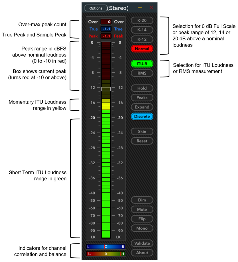
K-Meter by M. Zuther is example of software-based loudness meter
This meter can be shifted to a preferred place on the computer’s screen. It provides a Validate feature than can measure the Integrated Loudness of audio files at many times the normal playback speed.
In addition to familiar bar graph displays, some software-based loudness meters provide additional data about the audio. The Youlean Loudness Meter shown below has a number of numeric readouts flanked by a live bar graph on the left and a graphical display of loudness over time on the right.
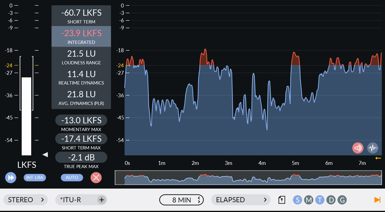
Youlean Loudness Meter includes numeric readouts and time display
The numeric display features (top to bottom, from the start of measurement) an average of Short-Term Loudness, Integrated Loudness, ITU Loudness Range, proprietary measurements of Realtime Dynamics and Average Dynamics, maximum Momentary Loudness, maximum Short-Term Loudness and True Peak maximum. The time graph shows Short Term Loudness over any desired period from a minute to hours and loudness exceeding the target value are displayed in red.
In addition to live monitoring, some loudness meters are available as software plug-ins for digital audio workstations (DAWs) or run standalone, allowing the measurement of loudness parameters of audio files.
A number of hardware meters have been developed for standalone operation. These meters are suited for operation on the bridge of a console or mixer and have convenient controls and measurement features.
When a digital signal is converted to analog, peaks can occur in the continuous time-domain signal between the digital samples. These are referred to as intersample peaks, and they can be substantially higher than the sample peaks observed in the digital domain. This chart shows an analog waveform where the digital samples do not fall on the actual peaks.
Analog waveform with digital samples (red dots)
Although intersample peaks are not obvious when looking at the digital signal, the digital signal actually does contain all the information about what happens in the continuous domain between the digital samples (this is a result of the Nyquist Sampling Theorem). True peak measurement estimates these intersample peaks so that overload can be avoided at later audio stages; if not addressed, these overloads could become audible distortion.
The intersample peaks between digital samples can be estimated in the digital domain by upsampling. ITU-R BS.1770 recommends upsampling by 4x (though it’s not necessary to go beyond 192 kHz), and then measuring the peak sample values from the up-sampled audio to get an estimate of the True Peak level.
Since the very beginning of audio recording and transmission, engineers had to deal with noise that degrades the quality of the intended audio signal. A great example is analog tape as a recording medium. To get the highest quality signal possible, the audio signal is increased so that the recorder noise (i.e., tape hiss) is as minimal as possible compared to the signal itself. If the recorded signal stays within the range of the tape’s magnetic potential, the recording and reproduction process is considered nearly linear. However, if a signal is increased too far, the physical medium cannot properly represent the peaks of the signal. Visualizing this signal, the peaks appear to be flatter than the original signal as depicted in Figure XX. This is a nonlinear distortion of the original signal, known as “soft clipping”, or sometimes referred to as “saturation”.
Digital audio signals on the other hand can be perfectly represented until full scale is reached. Once any digital samples exceed this maximum or minimum limit, those samples are truncated, which immediately “clips” the peaks. This immediate flattening is called “hard clipping”, as depicted below. Hard clipping quickly becomes audible and is considered harsher sounding than soft clipping.

Waveform with Various Types of Clipping
It should be noted that both soft clipping and hard clipping can be used creatively throughout the production chain, the classic example being a guitar amp cranked up to 11. Saturation and clipping distortion therefore are not bad per se – as long as they are not unwanted.
RMS, or the complicated-sounding term “root mean squared” is computed just like the name says:
For alternating current waveforms, such as audio, RMS measurement provides the equivalent direct current power in the waveform. This may be useful in determining how much power an amplifier draws to drive a loudspeaker. In audio metering, that is seldom an important matter. However, because RMS involves an average over time (of squared amplitudes), the duration of the average can be important in defining the ballistics of the audio meter. This slows the meter indication, making the meter easier to follow by eye.
Despite the smooth and slow movement, RMS metering has a drawback. Slowing the response speed of a meter causes a loss of audio signal peaks, which as discussed above are important in indicating and avoiding signal overload. Sometimes a small lamp was added in or near each RMS meter to indicate that some peak threshold had been reached. This gave only a single-valued indication, however, which might mean it was too late to do anything about the peak.
The VU meter was a popular audio display on broadcast and mixing consoles and audio recording equipment from the 1940’s until recent years. Its official name is the Standard Volume Indicator (SVI), with dB markings that measure program audio signal levels in “volume units”. The SVI is a simple averaging voltmeter with a moderate rise and fall time of about 300ms.
The VU meter began in 1938 as a collaborative project by CBS, NBC and Bell Telephone Laboratories, when the variety of audio meter types led to confusion and disagreement in the exchange of radio network programming. Extensive studies considered various metering techniques, including quasi-peak measurement. A paper published in 1940 reported that a moderate attack (or ‘integration’) time of about 300ms was preferred by users to minimize eye fatigue, and which showed little advantage in protecting against audible peak overload with vacuum tube amplifiers of the time. The authors noted that this integration time was most accurate in measuring program levels Bell Labs performed psychoacoustic testing with a variety of speech and music to confirm that the ballistics provided a good correlation with perceived loudness.
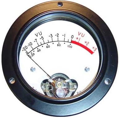
VU Meter with D’Arsonval (Moving Coil) Movement
An official VU meter has a mechanical pointer powered directly from the audio line it measures. The electrical internal design places the VU meter mid-way between a linear and root-mean-square detector. It therefore doesn’t fully have the energy-equivalence of an RMS meter. The meter/rectifier combination resulted in a scale range of approximately 23 VU (dB), which exceeded most other meters of the time.
A photo of the original meter with the “Type A” (VU on top) scale is shown above. For ease of reading, a color scheme of black scale and lettering on a “rich crème” background, with a thicker portion of the scale from 0 to +3 VU in red was selected. The meter was standardized in 1942 as ANSI specification “Volume Measurements of Electrical Speech and Program waves,” C16.5-1942 and is now incorporated into IEC Standard 60268-17.
As early as the 1930’s it was known that perception of loudness is frequency dependent. The famous curves in the figure below were published in 1933 by Fletcher and Munson of Bell Laboratories to show the sound pressure level needed for tones at each frequency to be perceived as equally loud.
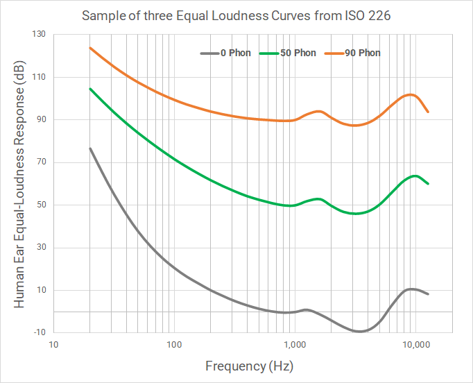
These curves are known as “equal loudness contours” and show that human hearing is most sensitive in the mid-high 2-5 kHz range, and increasingly less sensitive in the frequency range below 1000 Hz. For example, a 1000 Hz tone at 50 dB SPL and a 100 Hz tone at 70 dB SPL are on the same equal loudness contour. The curves are referred to in this figure in “phon” which is used by audiologists to provide a logarithmic measurement (like decibels) for perceived sound magnitude.
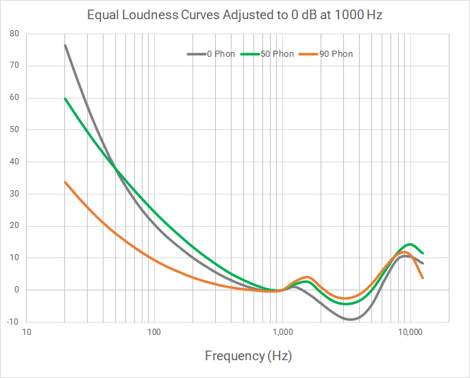
The shape of the equal loudness contours becomes flatter at higher playback levels, as shown the figure above. Note that as the sound pressures move from 0 Phon to 90 Phon that the curves become flatter, particularly on frequencies below 1000 Hz. This can be heard by playing the same track at a progressively higher levels that seemingly boosts very low frequencies relative to the midrange frequencies. Audio engineers have no way of knowing the ultimate playback level of listeners, thus the ITU Loudness model employs a single “K-weighting” curve. This weighting was adapted from a frequency loudness curve at 70 phon, which is generally considered the level chosen by television viewers. This is discussed further in the Learn More: K-weighting and other frequency weighting schemes.
Non-compliant (louder) streams may be perceived by some as initially attractive, but there are tradeoffs to the sonics!
Repeatedly it has been shown, that the same audio material is judged to be sounding initially attractive if purely its level is increased – even by a very small margin of for example 0.5 dB. This effect is one of the reasons for the increase in loudness levels over the past decades. As this happens subconsciously, it is a very important fact to know for anyone involved in the creation of audio content, from musicians to distributors, and applies to several stages of the production chain.
Besides in mixing and mastering, where obviously level differences are deliberately introduced and this effect should be accounted for, one must be aware that this effect can also take place in the distribution. Since there are multiple platforms and online broadcasts, who might stream the same piece of music, not all might be compliant with the current AES recommendations for streaming services.
Especially if the services are aiming at higher loudness levels, one might have the impression that the same piece of music sounds better than on other services. This conclusion is a misperception!
As the recommended levels have been carefully chosen, choosing higher levels for the own stream creates more disadvantages than advantages, such as unnecessary and harmful reduction of dynamic space. It limits the dynamic possibilities of content producers and/or artists and thus sacrifices their artistic freedom. Furthermore, such limited dynamic range will on average sound less pleasing to an audience compared to the same music with higher dynamic range if played back at the same loudness level. Other issues of not following the recommended practices were also discussed in the very first paragraph (What is loudness and why does it matter?).
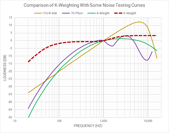
As explained in the Learn More: Equal loudness contours, human perception of loudness depends not only on frequency, but also on the overall sound pressure level being exposed to. Furthermore, there can be reasons to prioritize certain types of sound when applying frequency weighting. For these reasons, there’s no single way to define a frequency weighting curve that works in all scenarios.
Some technical curves (also called “contours”) were developed to measure environmental noise levels that could be annoying, such as traffic, while others are used to measure background sound such as building air conditioning, and even more were developed to measure electrical noise in radio and recording channels. A few such frequency weighting curves are shown in this figure, compared to the ITU Loudness “K-weighting” curve and the ear’s equal loudness contour at 70 Phon. All the curves are aligned for their magnitude responses to intersect at 0 dB at 1000 Hz.
This section provides a look inside the current loudness meter, based on Recommendation ITU-R BS.1770-4. The figure below shows the loudness meter in diagram form (LKFS is equivalent to LUFS). Actual designs may vary slightly, but this shows the key parts of the meter.
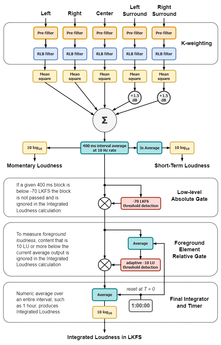
Audio enters at the top, showing a basic five-channel configuration (Left, Right, Center, Left Surround and Right Surround). A low frequency effects (LFE) input is not included as very low frequencies contribute little to perceptual loudness.
The first stage contains two filter blocks called the K-weighting filter, which approximates the frequency response of the human ear at normal playback levels. The Pre-filter provides a high frequency gain above 1 kHz that is shelved at approximately +4 dB above 3 kHz. The RLB filter is a simple high-pass filter with a second order rolloff below about 100 Hz. The combined response of these weighting networks is found in Learn More: K-weighting and other frequency weighting schemes
The mean square of the individual channels is performed here. In mathematics, the mean square is defined as the arithmetic mean of the squares of a set of numbers, so this step is part of a calculation of power over a specific time, performed in the step below. Before that, the mean square values of each channel are summed. Surround channels are given 1.5 dB of gain (a linear gain of 1.41) to account for their position nearer to each side of the listener, unlike to the Left, Right and Center channels that are some distance forward.
The mean squares of each channel (including a channel weighting for the surround channels) are summed and averaged over a 400 millisecond interval. All samples in the 400 ms interval are weighted equally. This channel summation is performed every 100 ms (10 Hz) which is an overlap of 75% of each 400 ms block.
After base-10 logarithmic conversion to output is available for a Momentary Loudness display, usually a moving bar graph. This display is popular with users but is visually active – similar to a VU meter. Its excursions may frequently run several dB higher than the long-term Integrated Loudness.
A second output is provided by 3-second averaging of the momentary measurements, called Short-Term Loudness. This measurement is visually smoother than Momentary Loudness and can be less tiring to watch, but more care may be needed to watch True Peak levels with higher-level content.
Integrated Loudness measurements may span relatively long periods (radio programs or movies can last an hour or more). As averaging is involved, periods of silence in the content will reduce the estimated loudness measurement. However, silence or a nearly silent part may have little subjective effect on long-term loudness: imagine a movie scene outside on a field, where two people are having a normal conversation with quiet crickets in the background. The dialogue is drawing our attention, so our loudness perception is dominated by the dialogue. The crickets on the other hand don’t contribute to the loudness impression and therefore should be ignored in the measurement as well.
The BS.1770 algorithm (added with the BS.1770-2 revision) includes a two-step gating approach. The first is a low-level absolute gate with a fixed threshold of -70 LKFS(LUFS), where only blocks above the threshold are passed to the Integrated Loudness calculation. The second step is a relative-level gate to focus on the foreground portion of the content. All the blocks that are above the low-level absolute gate are averaged and the resulting value is decreased by 10 LU and used as the gating threshold. All the blocks that exceed this gating threshold are passed to the final integrator.
This arrangement was found to solve the effects of quiet passages in movies biasing the overall loudness of a movies. However, the level of dialog may fall below this level gate in cases of wide dynamic range content, which could exclude the dialog from the overall Integrated Loudness.
The last stage performs an arithmetic average on the blocks that have successfully passed both gates. The average always begins at time zero and runs for a prescribed duration, however, in many implementations the loudness meters run in real time and the Integrated Loudness is continually updated over the interval.
The average results in a power of the pre-filtered and gated samples. The standard requires that the output be expressed in Loudness Units relative to full scale, or LUFS. This unit is equivalent to decibels, a base-10 logarithmic ratio, thus the last step is to perform a 10 log10 transform, and voilà, the Integrated Loudness is produced.
Notifications
